Most churn programmes rely on a binary ‘churn in 30 days’ flag. That makes decisions brittle, wastes data from still-active customers, and forces rework when business rules change. A better approach is to treat churn as time-based risk: generate a retention curve per customer so commercial teams can time interventions, choose 30/60/90-day windows at decision time without retraining, and allocate offers where uplift and unit economics justify the spend. 

In business terms, this improves revenue protection, LTV, and the ROI of retention activity by enabling teams to:

• Intervene earlier and more precisely, acting when customers are most at risk rather than at an arbitrary deadline
• Direct retention spend to where it pays back, balancing expected uplift, margin, and cost-to-serve
• Improve decisions using signals from all customers, not just those already labelled as churn risks
• Adapt quickly as rules change, shifting time horizons or policies without rebuilding models or relabelling data

In this article, we clarify what ‘leaving’ means in different business models, expose common pitfalls of binary labels, and show how a time-based risk view turns churn from a vague dashboard metric into actionable retention decisions, from pilot to production. 

What is churn, really? 

At its core, churn is about a customer stepping back from their relationship with you. What that looks like depends on your business model and customer journey. In different contexts, churn might be defined as:

• A subscription customer who cancels their contract
• A shopper who has not purchased anything for 30 days
• A device-based service with no active usage in the past week, with seasonal exceptions like Christmas

Each definition looks sensible in isolation; none is universal. The ambiguity is not just semantic; your mathematical target variable, the features you are allowed to use, and ultimately the ROI of any retention programme hang on this choice. To move from hand-waving to science we need to (a) make the hidden temporal assumptions explicit and (b) choose a modelling frame that reflects how customer lifecycles actually work over time. Below, we first disentangle the business and data-science angles, then borrow a concept from epidemiology, survival analysis, to show how the whole churn puzzle snaps into place. 

The business lens – three archetypes of ‘leaving’ 

Not all ‘leaving’ looks the same. Depending on your model, the churn moment, whether customers can return, and how you should measure it will all differ. The table below contrasts three practical archetypes – contract subscriptions, soft memberships, and usage‑based/retail – across the operative event, reversibility, and the KPI to anchor on. Use it to lock definitions up front, so labels, features, and success metrics line up with how your customers actually disengage and (sometimes) come back.

The data-science lens – why binary labels are a trap 

Binary labels feel natural because dashboards and CRM systems want a red/green light. What the business hears is “Give me a yes/no score so marketing can call the people in red.” Unfortunately, the moment we flatten customer behaviour into a crisp *churned / not-churned* stamp, we introduce a bunch of statistical problems that silently degrade every metric we report later.  

Below we unpack the most common traps.

The tyranny of τ

To make churn look binary we must pick a prediction horizon, τ, which yields the following classification problem: “Based on the history, will a customer churn within the next τ days?”

The typical rule for labelling when no explicit churn flag exists: “Mark a customer as churned if no purchase occurs within the next 30 days.”

The problems this creates are:

• Arbitrariness: thirty days suits fashion retail; seven days suits food delivery. Choose the wrong τ and the model optimises the wrong business question.
• Coupled pipelines: change τ and you have to relabel the whole history, retrain, revalidate, and reexplain the model.
• Data wastage: rows from the last τ days cannot yet be labelled, so the newest (often most valuable) customers are discarded.

A single integer ends up dictating both model accuracy and the company’s workflow, an inherently fragile situation. 

Right-censoring – information we throw away 

A plausible core assumption is that everybody will churn at some point in the future. Consequently, every customer who is still active today has an unknown time-to-churn; statisticians call this a right-censored observation. 

The standard binary setup deals with censored rows by dropping them. The result can lead to an older-than-reality training set, overly pessimistic risk estimates, and money wasted on data acquisition that is never used. 

Label leakage – the problem with looking into the future

A machine-learning model should be trained only on information that would have been available at the moment the prediction is made. Any statistic that sneaks in knowledge from the ‘future’ converts the training exercise into a retrospective classification game that the model will never be allowed to play in production. This phenomenon, as old as forecasting itself, is called information or label leakage. 

The churn label is defined by future inactivity. If we decide that “no purchase within the next 30 days” constitutes churn, the binary outcome for a record stamped 1 January depends on everything that happens until 31 January. However, many of the variables most useful for prediction are themselves aggregates over time: average spend, number of log-ins, last-session duration. Unless we are extremely strict about the window over which those aggregates are computed, they will contain events that occur after the prediction time and are therefore statistically entangled with the target. 

Customer activity exhibits strong positive serial correlation: the probability of an event at t + k conditional on an event at t decays slowly with k. The absence of events, what ultimately defines churn, is simply the lower tail of the same process. Any variable that counts, averages, or otherwise summarises behaviour across a window overlapping (t₀, t₀ + τ] will therefore share variance with the label. Without rigorous temporal cut-offs, feature engineering pipelines inevitably absorb that overlap and propagate it into the training matrix. This look-ahead bias can add several percentage points to AUC, and the posterior probabilities learned under leakage underestimate uncertainty because some explanatory power arose from ‘cheating’. 

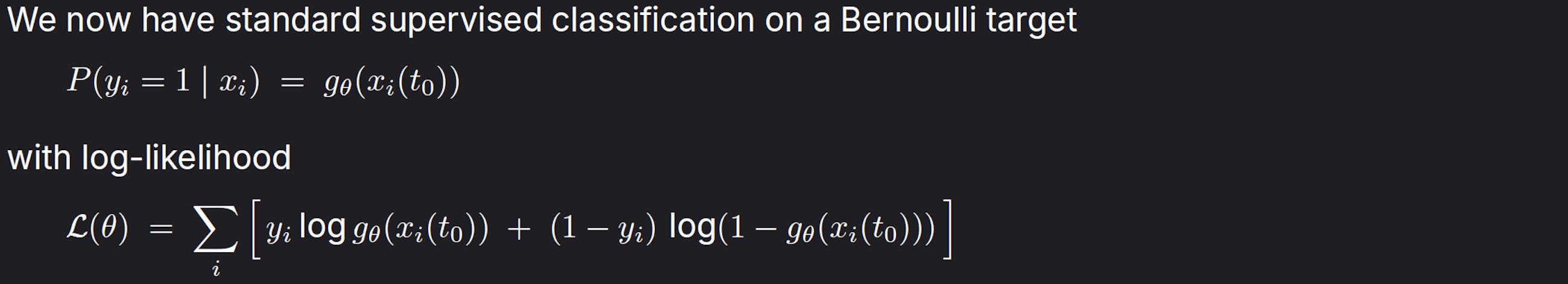
Training a classification model on churn / no-churn within τ 

That being said, there are some obvious benefits to using this definition. It is simple, relatively quick to build, and easy to explain. Additionally, we can choose whichever prediction algorithm we like, from logistic regression to decision-tree models to neural networks. Below is a breakdown of what that would look like: 

Labelling 

If we have no explicit churn event, but base churn on inactivity: 

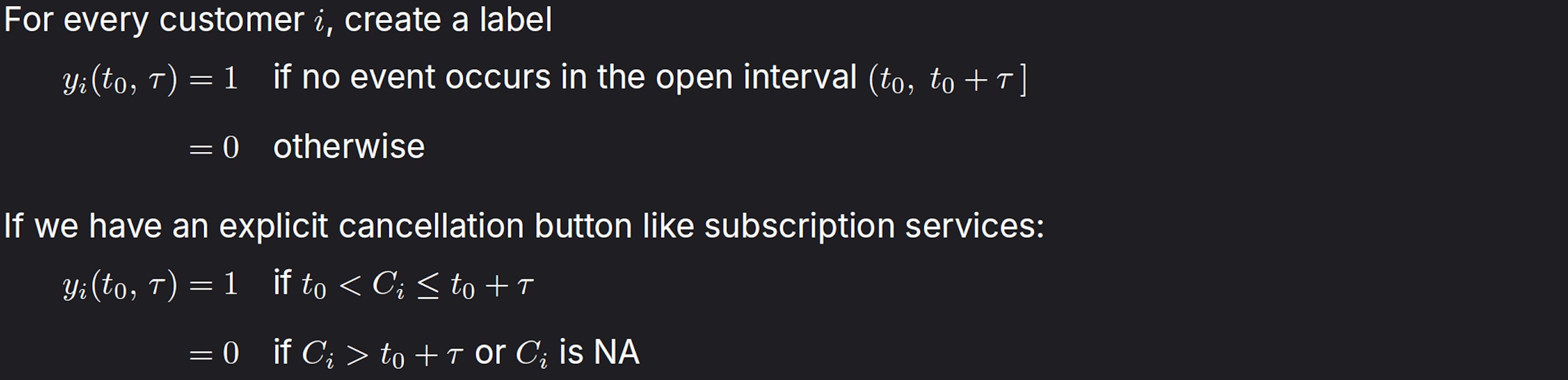
Here, however, τ is only a post-processing choice; the underlying data already contain the true event time. 

Feature engineering 

With yᵢ(t₀, τ) defined, the next step is to design features that capture meaningful signals up to the decision time t₀, carefully avoiding any look-ahead leakage. 

Compile a feature vector xᵢ(t₀) that uses only information available at or before t₀. 
These features may be static (country, segment) or dynamic (number of logins in the last seven days, recency, RFM scores, embeddings from click-streams). 

Statistical model 

Typical learning algorithms 

• Logistic regression or elastic-net GLM – interpretable coefficients
• Gradient-boosted decision trees (XGBoost, LightGBM, CatBoost) – industry work-horse; handles non-linearities and mixed data types
• Random forests – robust to multicollinearity, little tuning
• Feed-forward or recurrent neural nets
• Calibration layers (Platt scaling, isotonic regression) often added post-hoc because raw scores are rarely well-calibrated

Evaluation metrics 

Start with how you’ll use the scores; rank customers, set a threshold, or use calibrated probabilities and choose metrics accordingly: 

• Ranking quality: Use AUC/ROC for overall ordering; prefer PR-AUC and precision@k in imbalanced settings
• Probability quality: Optimise log-loss; verify calibration with reliability plots; apply post-hoc calibration (Platt scaling, isotonic regression) on a holdout set if needed
• Thresholded decisions: Report precision, recall, and F1 at the chosen operating point; pick the threshold by maximising expected profit or honouring capacity constraints

Business teams usually overlay profit curves because the label itself is an all-or-nothing abstraction. 

Key mathematical limitations

• The label depends on τ; changing τ alters both the loss function and the training sample
• Right-censored cases (customers still active) contribute no likelihood and therefore no information
• The model produces one probability for one τ; it cannot answer “what is the risk at 60 days vs 90 days?” without retraining

There is another way: treat churn as a time-to-event question, learn from every customer – including the ones still happily paying – and let the model output a full risk curve instead of a blunt yes/no for an arbitrary time horizon. 

Enter survival analysis – an analogy 

Imagine an oncologist following 1000 patients from diagnosis to either relapse or the study’s end date.

Event = relapse 
Clock starts = diagnosis day 
Outcome we care about = time (in months) until relapse 

Patients who are still healthy when the trial stops do not disappear from the data; they contribute partial information: 

“Patient is relapse-free for at least 24 months.” 

Statisticians call this right-censoring. Survival models are designed to ingest both fully observed and censored records without bias. 

Now replace patient with subscriber:

Event = next successful payment 
Clock starts = any point in the subscription timeline (often ‘now’) 
Outcome = days until the next payment 

A customer who paid yesterday and is still active contributes: 
“Subscriber will stay for at least one day; exact time to next payment unknown.” 

Ignoring these rows is equivalent to a hospital throwing away every living patient’s file before fitting a relapse model. You would not trust that oncologist; do not trust a churn model that drops recent customers. 

Customer A  |──────●──────────────●────?    (two payments observed, still active)

Customer B  |──────●────●──X                    (cancelled → event fully observed)

Customer C  |───●──────────────?             (one payment, no further data yet)

A survival model learns from all three customers:

– For A and C, it gets a lower bound on the waiting time. 
– For B, it knows the exact lifetime up to churn.

Using a survival definition of churn fixes:

1. Business interpretability – You speak the language of “probability the customer is still active after 30/60/90 days”.
2. No arbitrary horizon – The model outputs a full survival function; marketing can choose any cut-off after the fact.
3. Data efficiency – Every active customer provides a usable training signal from day one; no more discarding the freshest cohorts.
4. Consistency across segments – Whether a customer can ‘come back’ is naturally captured: the model sees a new event and simply resets the clock. No relabelling gymnastics required. 

Time-to-event modelling

Evaluation metrics: 

• Concordance index (Harrell’s C) – continuous analogue of AUC based on risk ordering
• Integrated Brier score – proper scoring rule for survival probabilities
• Calibration curves for Ŝ(t) vs. Kaplan-Meier
• Business-oriented: expected LTV, retention curve fit, incremental profit under selected intervention windows (any τ can be computed from the same model)

Mathematical strengths: 

• Censoring handled in the likelihood; no loss of information
• One fitted model yields Ŝ(t) for all t, so marketing can set different horizons without retraining
• When combined with time-varying x(t), the model becomes a continuous-time analogue of a recurrent classifier, capturing behavioural evolution instead of a snapshot 

Practical summary 

Binary classification with a fixed horizon τ is easy to deploy and compatible with generic ML tooling, but it encodes a hard assumption about when churn matters and degrades whenever τ changes or censoring is large. 

Time-to-event modelling treats churn as a stochastic clock. It uses every record, event, or censor, and returns a full survival curve from which any binary metric can be derived post-hoc. The price is higher conceptual complexity and the need for specialised libraries, but the mathematical foundations align better with how churn actually unfolds in the real world. 

So what? Implications for business teams 

• Targeting and timing
  • Move from “who is red today?” to “who is most at risk in the next 7/30/90 days, and when should we act?”
  • Stagger outreach around the peak hazard (when risk accelerates), smoothing contact centre load and improving take‑up
• Offer economics
  • Size incentives by expected value: offer only where expected LTV preserved minus cost is positive
  • Escalate interventions over time (soft nudges → discounts) based on the individual risk curve
• Capacity and planning
  • Allocate finite outreach capacity to the top risk‑adjusted opportunities each day/week
  • Set portfolio‑level policies (e.g., max offers per segment per week) without retraining models
• Reporting and governance
  • Track retention curves and expected revenue at 30/60/90 days per cohort and segment
  • Make policy changes (e.g., new grace periods) in the decision layer, not the modelling layer

Implications for data and engineering teams

• Data requirements
  • Reliable timestamps for events (purchases, logins, payments, cancellations) and clear definitions of inactivity‑based churn
  • Feature store with time‑travel/snapshotting to avoid leakage; explicit handling of reactivations
• Modelling approach
  • Keep a simple binary model as a baseline; add a survival model (Cox, Weibull/AFT, RSF/GBM‑Survival, or WTTE‑RNN for sequences)
  • Use time‑based splits, Harrell’s C / Integrated Brier Score, and calibration checks against Kaplan‑Meier
• Serving and integration
  • Expose S(t|x) and hazard h(t) via an API; compute risk at any business horizon on demand
  • Implement a rules/policy layer that maps risk and LTV to actions (e.g., contact, channel, offer)
• Monitoring and MLOps
  • Track drift in covariates, censoring mix, and calibration of risk at key horizons
  • Recalibrate or retrain on schedule or when calibration/error exceeds thresholds; keep label‑delay

If you treat churn as a time-to-event risk, you unlock powerful new insights and actions. You learn from every customer, not just those who have left; you get calibrated survival curves that let teams pick any 7/30/90-day horizon at decision time, time outreach around peak hazard, and price offers based on true expected value. The result is a resilient retention engine, fewer relabelling gymnastics, better use of fresh data, and auditable, profit-aware decisions that hold up as policies and seasons change. In short, survival thinking turns churn from a brittle dashboard flag into a scalable, production-ready playbook.